When you copy a cell containing a formula, you will notice that the cell references in the formula also move a corresponding number of cells across and down. This type of cell reference is called a relative reference.
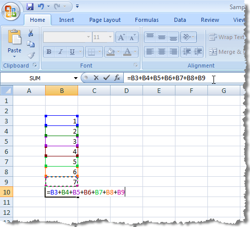
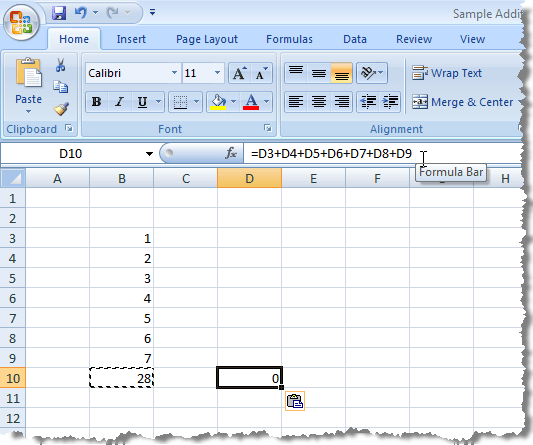
When we copy (Ctrl + C) the formula in the image above, and paste (Ctrl + V) it into another cell, you’ll notice that the cell references change from the B column to the D column, so the total is different.
If you want to prevent Excel from changing the cell references when copying cells, you need to use absolute references. To create an absolute reference, insert a dollar sign ($) before both parts of the cell reference in the formula you want to freeze, as illustrated in the following image.
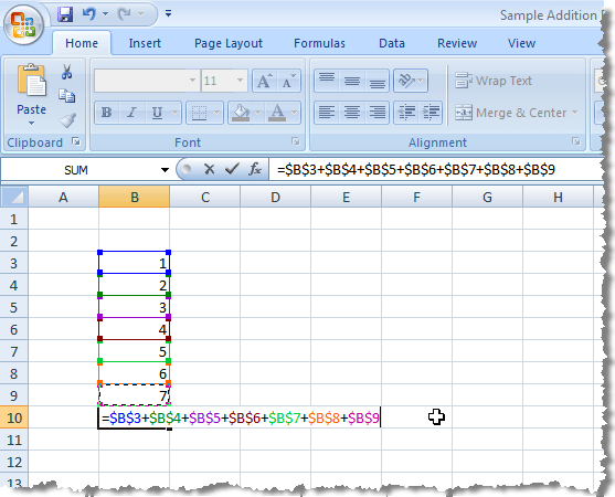
There are three different types of references, relative, absolute, and mixed. The following are some examples:
- Relative Reference: A1 tells Excel to change the cell references to the corresponding columns and rows.
- Mixed Reference: $A1 tells Excel you always want to refer to column A.
- Mixed Reference: B$1 tells Excel you always want to refer to row 1.
- Absolute Reference: $B$1 tells Excel you always want to refer to cell B1.
There is a shorthand method for entering the dollar signs as you select or enter cell references in a formula. As you are typing a formula and finish a cell reference, press F4 to toggle between the 4 combinations of reference types. Let’s say you started typing a formula and you typed =100*B1.
- Press F4 and your formula changes to =100*$B$1 (always refer to cell B1)
- Press F4 again and your formula changes to =100*B$1 (always refer to row 1)
- Press F4 again and your formula changes to =100*$B1 (always refer to column B)
- Press F4 again and your formula returns to the original relative reference =100*B1 (always change the reference to the corresponding columns and rows)
You can pause while entering each cell reference in the formula to press F4 until you get the right reference type for the current cell reference.
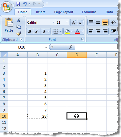
To copy the formula entered using absolute references and preserve the cell references, select the cell containing the formula and copy it (Ctrl + C) and click the destination cell into which you want to paste the formula.
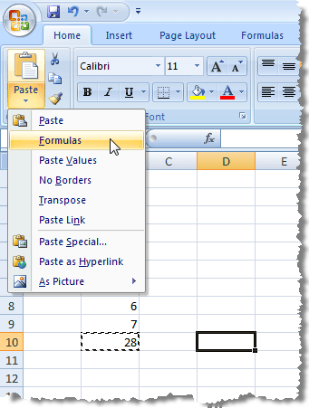
Make sure the Home tab is the active tab on the ribbon. Click the arrow on the Paste button in the Paste section of the Home tab. Select Formulas from the drop-down menu.
You will notice that the total displays in the destination cell from the original cell, and the formula that displays in the Formula Bar for the destination cell contains the same absolute references as the original formula in the original cell.
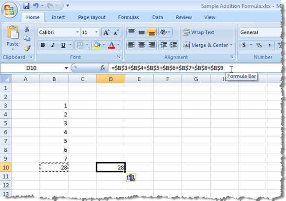
NOTE: Copying and pasting a formula into a destination cell does not mean that the formula will be updated in the destination cell when it is updated in the original cell.
There is a way you can copy and paste a cell containing a formula to a destination cell such that the results of the formula in the original cell always display in the destination cell as they change. You can link to the original cell.
To do this, select and copy the original cell with the formula again and click the cell into which you want to paste the link to the original cell. Click the Paste button in the Paste section of the Home tab to display the drop-down menu. Select Paste Link from the menu.
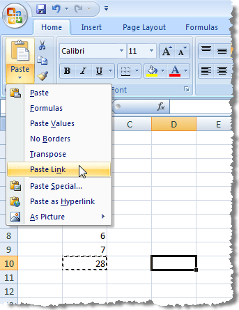
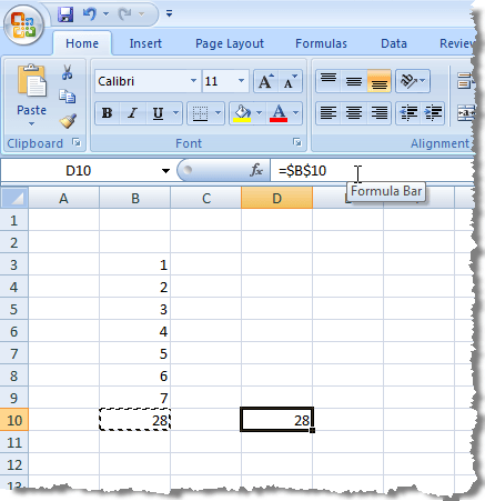
You will notice that, again, the total from the original cell displays in the destination cell. However, this time, the Formula Bar displays an absolute reference to the original cell containing the formula. Every time the results change in the original cell, the total displayed in the destination cell updates as well.
NOTE: If all you want to do is paste the result of the formula into the destination cell, select Paste Values from the Paste drop-down menu when pasting into the destination cell.
Pasting a link is a handy feature if you want to display a total from one part of a worksheet in a more prominent location with special formatting, possibly for a presentation, and you want to keep the cell containing the link updated. Enjoy!

